Introduction
This post is simply a sandbox/cookbook of R code I’m exploring for common healthcare aging of accounts-related analyses.
Packages
Data
# Sheet is public and shareable
gs4_deauth()

# Google Sheet ID
id_aging <- "1Td3_6sYOEVwSOdaWdBeUl8yLUp7ztFu8tesZ6LcLlv4"

# Read in Google Sheet
google_aging <- read_sheet(ss = id_aging, sheet = "Sheet1")

# Convert Date of Service column to date object
google_aging$dos <- as.Date(google_aging$dos, "%m/%d/%Y")

# Print head of data
paged_table(google_aging)
# Add Age Column
google_aging <- google_aging |>
mutate(age = days(Sys.Date()) - days(dos))
google_aging$age <- as.numeric(google_aging$age, "hours")
google_aging <- google_aging |>
mutate(age = age / 24)
# Add Bucket Column
google_aging <- google_aging |>
mutate(bucket = case_when(
age < 31 ~ "0-30",
age >= 31 & age < 61 ~ "31-60",
age >= 61 & age < 91 ~ "61-90",
age >= 91 & age < 121 ~ "91-120",
age >= 121 & age < 151 ~ "121-150",
age >= 151 & age < 181 ~ "151-180",
age >= 181 ~ "181+",
TRUE ~ "UNKNOWN"
))
google_aging$bucket <- factor(google_aging$bucket,
levels = c(
"0-30", "31-60", "61-90",
"91-120", "121-150", "151-180",
"181+", "UNKNOWN"
),
ordered = is.ordered(google_aging$bucket)
)
# Print head of data
paged_table(google_aging)# Add 'filelimit' Column
google_aging <- google_aging |>
mutate(filelimit = case_when(
payer == "AETNA" ~ "180",
payer == "Ambetter" ~ "180",
payer == "Blue Cross" ~ "365",
payer == "CIGNA" ~ "90",
payer == "Coventry" ~ "180",
payer == "Humana" ~ "90",
payer == "Medicaid" ~ "180",
payer == "Medicare" ~ "365",
payer == "Meritain" ~ "90",
payer == "UHC" ~ "90",
payer == "Patient" ~ "0",
TRUE ~ "Other"
))
## Convert 'filelimit' Column to Numeric
google_aging$filelimit <- as.numeric(google_aging$filelimit)
## Add 'filelimdate' Column - Age of Claim
google_aging <- google_aging |>
mutate(filelimdate = case_when(
filelimit > 0 ~ as.Date(dos) + days(filelimit),
TRUE ~ as.Date(dos)
))
## Add 'filelimdays' Column - Age of Claim
google_aging <- google_aging |>
mutate(filelimdays = case_when(
filelimit > 0 ~ filelimit - age,
TRUE ~ 5000 # dummy variable for Patient Class
))
# Print head of data
paged_table(google_aging)Visualizations
Bar/Column Charts
Code
google_aging |>
  group_by(bucket) |>
  summarise(
    total = sum(amt),
    encounters = n()
  ) |>
  hchart(
    "column",
    hcaes(bucket, round(encounters, 0), color = bucket)
  ) |>
  hc_yAxis(
    gridLineWidth = 0,
    labels = list(style = list(color = "#000000")),
    title = list(text = " ", style = list(color = "#000000"))
  ) |>
  hc_xAxis(
    labels = list(style = list(color = "#000000")),
    title = list(text = " "),
    lineWidth = 0,
    tickWidth = 0
  ) |>
  hc_title(text = "Number of Encounters by Bucket") |>
  hc_add_theme(hc_theme_smpl()) |>
  hc_tooltip(
    useHTML = TRUE,
    crosshairs = TRUE,
    borderWidth = 1,
    sort = TRUE
  ) |>
  hc_plotOptions(
    column = list(
      dataLabels = list(
        valueDecimals = 0,
        enabled = TRUE
      )
    )
  ) |>
  hc_size(height = 400, width = 800)
Code
google_aging |>
  group_by(bucket, payer) |>
  summarise(
    total = sum(amt),
    encounters = n()
  ) |>
  hchart(
    "column",
    hcaes(bucket, round(encounters, 0), group = payer, color = payer)
  ) |>
  hc_yAxis(
    gridLineWidth = 0,
    labels = list(style = list(color = "#000000")),
    title = list(text = " ", style = list(color = "#000000"))
  ) |>
  hc_xAxis(
    labels = list(style = list(color = "#000000")),
    title = list(text = " "),
    lineWidth = 0,
    tickWidth = 0
  ) |>
  hc_title(text = "Number of Encounters Per Payer by Bucket") |>
  hc_add_theme(hc_theme_smpl()) |>
  hc_tooltip(
    useHTML = TRUE,
    crosshairs = TRUE,
    borderWidth = 1,
    sort = TRUE
  ) |>
  hc_plotOptions(
    column = list(
      dataLabels = list(
        valueDecimals = 0,
        enabled = TRUE
      )
    )
  ) |>
  hc_size(height = 400, width = 800)
Code
google_aging |>
  group_by(payer, bucket) |>
  summarise(
    total = sum(amt),
    encounters = n()
  ) |>
  hchart(
    "bar",
    hcaes(bucket, round(total, 0), group = payer)
  ) |>
  hc_yAxis(
    gridLineWidth = 0,
    labels = list(style = list(color = "#000000")),
    title = list(text = " ", style = list(color = "#000000"))
  ) |>
  hc_xAxis(
    labels = list(style = list(color = "#000000")),
    title = list(text = " "),
    lineWidth = 0,
    tickWidth = 0
  ) |>
  hc_title(text = "Dollar Amount by Bucket Per Payer") |>
  hc_add_theme(hc_theme_smpl()) |>
  hc_tooltip(
    useHTML = TRUE,
    crosshairs = TRUE,
    borderWidth = 1,
    sort = TRUE
  ) |>
  hc_plotOptions(
    column = list(
      dataLabels = list(
        valueDecimals = 0,
        enabled = TRUE
      )
    )
  ) |>
  hc_size(height = 600, width = 800)
Linear Regression Plots
aging_bailey <- google_aging |>
  filter(provider == "Bailey")

splot(amt ~ age * payer * referring_phys, aging_bailey)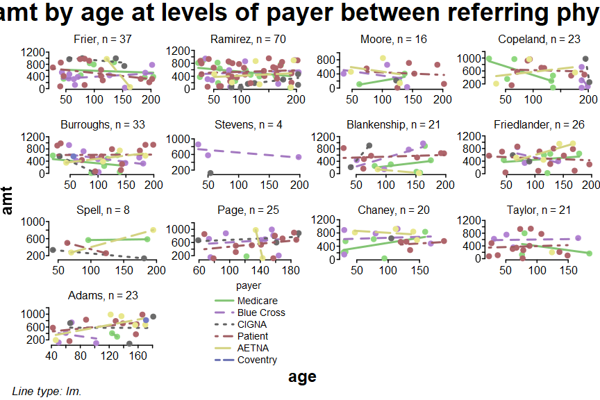
Code
hchart(
  aging_bailey,
  "scatter",
  hcaes(x = age, y = amt, group = payer),
  regression = TRUE
) |>
  hc_add_theme(hc_theme_smpl()) |>
  hc_add_dependency("plugins/highcharts-regression.js") |>
  hc_size(height = 1000)
Code
hchart(google_aging, "scatter",
  hcaes(x = age, y = amt, group = provider),
  regression = TRUE
) |>
  hc_add_theme(hc_theme_smpl()) |>
  hc_add_dependency("plugins/highcharts-regression.js") |>
  hc_size(height = 1000, width = 800)
Relationship Visualizations
refer2prov <- google_aging |>
  dplyr::group_by(referring_phys, provider) |>
  dplyr::summarise(count = n()) |>
  dplyr::arrange(desc(count)) |>
  ungroup() |>
  rename(from = referring_phys, to = provider, weight = count)
refer2prov
# # A tibble: 65 × 3
# from to weight
# <chr> <chr> <int>
# 1 Ramirez James 177
# 2 Ramirez Forrest 131
# 3 Ramirez Timothy 117
# 4 Blankenship James 76
# 5 Burroughs James 75
# 6 Ramirez Bailey 70
# 7 Frier James 69
# 8 Page James 66
# 9 Burroughs Forrest 65
# 10 Ramirez Allen 64
# # … with 55 more rows
# # ℹ Use `print(n = ...)` to see more rowsprov2payer <- google_aging |>
dplyr::group_by(provider, payer) |>
dplyr::summarise(count = n()) |>
dplyr::arrange(desc(count)) |>
ungroup() |>
rename(from = provider, to = payer, weight = count)
prov2payer# # A tibble: 30 × 3
# from to weight
# <chr> <chr> <int>
# 1 James Patient 308
# 2 Forrest Patient 268
# 3 Timothy Patient 206
# 4 James Blue Cross 170
# 5 James Medicare 156
# 6 Forrest Blue Cross 133
# 7 Bailey Patient 128
# 8 Forrest Medicare 126
# 9 Allen Patient 113
# 10 Timothy Blue Cross 113
# # … with 20 more rows
# # ℹ Use `print(n = ...)` to see more rowsref2prov2pay <- rbind(refer2prov, prov2payer)
ref2prov2pay# # A tibble: 95 × 3
# from to weight
# <chr> <chr> <int>
# 1 Ramirez James 177
# 2 Ramirez Forrest 131
# 3 Ramirez Timothy 117
# 4 Blankenship James 76
# 5 Burroughs James 75
# 6 Ramirez Bailey 70
# 7 Frier James 69
# 8 Page James 66
# 9 Burroughs Forrest 65
# 10 Ramirez Allen 64
# # … with 85 more rows
# # ℹ Use `print(n = ...)` to see more rowsSankey Diagram
Dependency Wheel
Vtree Visualizations
vtree(
  google_aging,
  "referring_phys",
  horiz = FALSE,
  title = "Encounters",
  height = "50%",
  width = "100%",
  rounded = FALSE,
  showvarnames = FALSE,
  pngknit = FALSE,
  pattern = FALSE
)
Misc Visualizations
Sunburst Chart
with {sunburstR}
Code
aging_df <- data.frame(
  level1 = rep(c("Primary", "Secondary"), each = 7),
  level2 = rep(c(
    "Cigna",
    "BCBS",
    "Medicare",
    "Aetna",
    "Humana",
    "UHC",
    "Medicaid"
  ), 2),
  size = c(
    101586.44, 813932.10, 244682.06,
    315442.09, 338892.56, 692951.00,
    172394.44, 30869.21, 75555.29,
    12601.41, 39003.59, 27713.18,
    14384.15, 222480.09
  ),
  stringsAsFactors = FALSE
)
aging_df
# level1 level2 size
# 1 Primary Cigna 101586.44
# 2 Primary BCBS 813932.10
# 3 Primary Medicare 244682.06
# 4 Primary Aetna 315442.09
# 5 Primary Humana 338892.56
# 6 Primary UHC 692951.00
# 7 Primary Medicaid 172394.44
# 8 Secondary Cigna 30869.21
# 9 Secondary BCBS 75555.29
# 10 Secondary Medicare 12601.41
# 11 Secondary Aetna 39003.59
# 12 Secondary Humana 27713.18
# 13 Secondary UHC 14384.15
# 14 Secondary Medicaid 222480.09# 'json' chr "{\"children\":[{\"name\":\"Primary\",\"children\":[{\"name\":\"Cigna\",\"size\":101586.44,\"colname\":\"level2\"| __truncated__Code
library(sunburstR)

sb1 <- sunburst(tree, width = "100%", height = 600)

sb3 <- sund2b(
  tree,
  width = "100%",
  height = 600,
  rootLabel = "Aging",
  showLabels = T,
  breadcrumbs = sund2bBreadcrumb(enabled = T),
  colors = list(range = RColorBrewer::brewer.pal(9, "Paired"))
)

div(
  style = "display: flex; align-items:center;",
  div(style = "width:50%; border:1px solid #ccc;", sb1),
  div(style = "width:50%; border:1px solid #ccc;", sb3)
)Drilldown Piechart
with {echarts4r}
Code
aging_df2 <- data.frame(
  parents = c(
    "",
    "Primary", "Primary",
    "Primary", "Primary",
    "Primary", "Primary", "Primary",
    "Secondary", "Secondary",
    "Secondary", "Secondary",
    "Secondary", "Secondary", "Secondary",
    "Everything", "Everything"
  ),
  labels = c(
    "Everything",
    "Cigna", "BCBS", "Medicare",
    "Aetna", "Humana", "UHC",
    "Medicaid", "Cigna", "BCBS",
    "Medicare", "Aetna", "Humana",
    "UHC", "Medicaid",
    "Primary", "Secondary"
  ),
  value = c(
    0,
    101586.44, 813932.10, 244682.06,
    315442.09, 338892.56, 692951.00,
    172394.44, 30869.21, 75555.29,
    12601.41, 39003.59, 27713.18,
    14384.15, 222480.09, 2679880.7,
    422606.9
  )
)

aging_df2
# parents labels value
# 1 Everything 0.00
# 2 Primary Cigna 101586.44
# 3 Primary BCBS 813932.10
# 4 Primary Medicare 244682.06
# 5 Primary Aetna 315442.09
# 6 Primary Humana 338892.56
# 7 Primary UHC 692951.00
# 8 Primary Medicaid 172394.44
# 9 Secondary Cigna 30869.21
# 10 Secondary BCBS 75555.29
# 11 Secondary Medicare 12601.41
# 12 Secondary Aetna 39003.59
# 13 Secondary Humana 27713.18
# 14 Secondary UHC 14384.15
# 15 Secondary Medicaid 222480.09
# 16 Everything Primary 2679880.70
# 17 Everything Secondary 422606.90# create a tree object
etree <- data.tree::FromDataFrameNetwork(aging_df2)
etree# levelName
# 1
# 2 °--Everything
# 3 ¦--Primary
# 4 ¦ ¦--Cigna
# 5 ¦ ¦--BCBS
# 6 ¦ ¦--Medicare
# 7 ¦ ¦--Aetna
# 8 ¦ ¦--Humana
# 9 ¦ ¦--UHC
# 10 ¦ °--Medicaid
# 11 °--Secondary
# 12 ¦--Cigna
# 13 ¦--BCBS
# 14 ¦--Medicare
# 15 ¦--Aetna
# 16 ¦--Humana
# 17 ¦--UHC
# 18 °--MedicaidSankey Diagram
in {echarts4r}
Citations
| Package | Version | Citation |
|---|---|---|
| base | 4.2.1 | R Core Team (2022) |
| d3r | 1.0.0 | Bostock, Russell, et al. (2021) |
| data.tree | 1.0.0 | Glur (2020) |
| distill | 1.4 | Dervieux et al. (2022) |
| echarts4r | 0.4.4 | Coene (2022) |
| grateful | 0.1.11 | Rodríguez-Sánchez, Jackson, and Hutchins (2022) |
| highcharter | 0.9.4 | Kunst (2022) |
| htmltools | 0.5.2 | Cheng et al. (2021) |
| htmlwidgets | 1.5.4 | Vaidyanathan et al. (2021) |
| knitr | 1.39 | Xie (2014); Xie (2015); Xie (2022) |
| RColorBrewer | 1.1.3 | Neuwirth (2022) |
| rmarkdown | 2.14 | Xie, Allaire, and Grolemund (2018); Xie, Dervieux, and Riederer (2020); Allaire et al. (2022) |
| sessioninfo | 1.2.2 | Wickham et al. (2021) |
| splot | 0.5.2 | Iserman (2022) |
| sunburstR | 2.1.6 | Bostock, Rodden, et al. (2021) |
| tidytable | 0.8.0 | Fairbanks (2022) |
| tidyverse | 1.3.1 | Wickham et al. (2019) |
| vtree | 5.4.6 | frame) (2021) |
| xaringanExtra | 0.7.0 | Aden-Buie and Warkentin (2022) |
Last updated on
# [1] "2022-07-19 12:14:07 EDT"Session Info
sessioninfo::session_info()# ─ Session info ───────────────────────────────────────────────────────────────────────────────────────────────────────────────────────────────────────────────────────────────────────────────────────
# setting value
# version R version 4.2.1 (2022-06-23 ucrt)
# os Windows 10 x64 (build 25158)
# system x86_64, mingw32
# ui RTerm
# language (EN)
# collate English_United States.utf8
# ctype English_United States.utf8
# tz America/New_York
# date 2022-07-19
# pandoc 2.17.1.1 @ C:/Program Files/RStudio/bin/quarto/bin/ (via rmarkdown)
#
# ─ Packages ───────────────────────────────────────────────────────────────────────────────────────────────────────────────────────────────────────────────────────────────────────────────────────────
# package * version date (UTC) lib source
# assertthat 0.2.1 2019-03-21 [1] CRAN (R 4.2.0)
# backports 1.4.1 2021-12-13 [1] CRAN (R 4.2.0)
# broom 1.0.0 2022-07-01 [1] CRAN (R 4.2.1)
# bslib 0.4.0 2022-07-16 [1] CRAN (R 4.2.1)
# cachem 1.0.6 2021-08-19 [1] CRAN (R 4.2.0)
# cellranger 1.1.0 2016-07-27 [1] CRAN (R 4.2.0)
# cli 3.3.0 2022-04-25 [1] CRAN (R 4.2.0)
# colorspace 2.0-3 2022-02-21 [1] CRAN (R 4.2.0)
# crayon 1.5.1 2022-03-26 [1] CRAN (R 4.2.0)
# curl 4.3.2 2021-06-23 [1] CRAN (R 4.2.0)
# d3r * 1.0.0 2022-04-26 [1] Github (timelyportfolio/d3r@f77d0a0)
# data.table 1.14.2 2021-09-27 [1] CRAN (R 4.2.0)
# data.tree 1.0.0 2020-08-03 [1] CRAN (R 4.2.1)
# DBI 1.1.3 2022-06-18 [1] CRAN (R 4.2.0)
# dbplyr 2.2.1 2022-06-27 [1] CRAN (R 4.2.0)
# DiagrammeR 1.0.9 2022-03-05 [1] CRAN (R 4.2.0)
# digest 0.6.29 2021-12-01 [1] CRAN (R 4.2.0)
# distill 1.4 2022-05-12 [1] CRAN (R 4.2.0)
# downlit 0.4.2 2022-07-05 [1] CRAN (R 4.2.0)
# dplyr * 1.0.9 2022-04-28 [1] CRAN (R 4.2.0)
# echarts4r * 0.4.4 2022-05-28 [1] CRAN (R 4.2.0)
# ellipsis 0.3.2 2021-04-29 [1] CRAN (R 4.2.0)
# evaluate 0.15 2022-02-18 [1] CRAN (R 4.2.0)
# fansi 1.0.3 2022-03-24 [1] CRAN (R 4.2.0)
# fastmap 1.1.0 2021-01-25 [1] CRAN (R 4.2.0)
# forcats * 0.5.1 2021-01-27 [1] CRAN (R 4.2.0)
# fs 1.5.2 2021-12-08 [1] CRAN (R 4.2.0)
# gargle 1.2.0.9002 2022-06-05 [1] Github (r-lib/gargle@1e67aa0)
# generics 0.1.3 2022-07-05 [1] CRAN (R 4.2.0)
# ggplot2 * 3.3.6 2022-05-03 [1] CRAN (R 4.2.0)
# glue 1.6.2 2022-02-24 [1] CRAN (R 4.2.0)
# googledrive 2.0.0 2021-07-08 [1] CRAN (R 4.2.0)
# googlesheets4 * 1.0.0 2021-07-21 [1] CRAN (R 4.2.0)
# grateful * 0.1.11 2022-05-07 [1] Github (Pakillo/grateful@ba9b003)
# gtable 0.3.0 2019-03-25 [1] CRAN (R 4.2.0)
# haven 2.5.0 2022-04-15 [1] CRAN (R 4.2.0)
# highcharter * 0.9.4 2022-01-03 [1] CRAN (R 4.2.0)
# highr 0.9 2021-04-16 [1] CRAN (R 4.2.0)
# hms 1.1.1 2021-09-26 [1] CRAN (R 4.2.0)
# htmltools * 0.5.2 2021-08-25 [1] CRAN (R 4.2.0)
# htmlwidgets * 1.5.4 2021-09-08 [1] CRAN (R 4.2.0)
# httpuv 1.6.5 2022-01-05 [1] CRAN (R 4.2.0)
# httr 1.4.3 2022-05-04 [1] CRAN (R 4.2.0)
# igraph 1.3.2 2022-06-13 [1] CRAN (R 4.2.1)
# jquerylib 0.1.4 2021-04-26 [1] CRAN (R 4.2.0)
# jsonlite 1.8.0 2022-02-22 [1] CRAN (R 4.2.0)
# knitr * 1.39 2022-04-26 [1] CRAN (R 4.2.0)
# later 1.3.0 2021-08-18 [1] CRAN (R 4.2.0)
# lattice 0.20-45 2021-09-22 [2] CRAN (R 4.2.1)
# lifecycle 1.0.1 2021-09-24 [1] CRAN (R 4.2.0)
# lubridate * 1.8.0 2021-10-07 [1] CRAN (R 4.2.0)
# magrittr 2.0.3 2022-03-30 [1] CRAN (R 4.2.0)
# memoise 2.0.1 2021-11-26 [1] CRAN (R 4.2.0)
# mime 0.12 2021-09-28 [1] CRAN (R 4.2.0)
# modelr 0.1.8 2020-05-19 [1] CRAN (R 4.2.0)
# munsell 0.5.0 2018-06-12 [1] CRAN (R 4.2.0)
# pillar 1.8.0 2022-07-18 [1] CRAN (R 4.2.1)
# pkgconfig 2.0.3 2019-09-22 [1] CRAN (R 4.2.0)
# promises 1.2.0.1 2021-02-11 [1] CRAN (R 4.2.0)
# purrr * 0.3.4 2020-04-17 [1] CRAN (R 4.2.0)
# quantmod 0.4.20 2022-04-29 [1] CRAN (R 4.2.0)
# R.cache 0.15.0 2021-04-30 [1] CRAN (R 4.2.0)
# R.methodsS3 1.8.2 2022-06-13 [1] CRAN (R 4.2.0)
# R.oo 1.25.0 2022-06-12 [1] CRAN (R 4.2.0)
# R.utils 2.12.0 2022-06-28 [1] CRAN (R 4.2.0)
# R6 2.5.1 2021-08-19 [1] CRAN (R 4.2.0)
# RColorBrewer 1.1-3 2022-04-03 [1] CRAN (R 4.2.0)
# Rcpp 1.0.9 2022-07-08 [1] CRAN (R 4.2.1)
# readr * 2.1.2 2022-01-30 [1] CRAN (R 4.2.0)
# readxl 1.4.0 2022-03-28 [1] CRAN (R 4.2.0)
# rematch2 2.1.2 2020-05-01 [1] CRAN (R 4.2.0)
# renv 0.15.5 2022-05-26 [1] CRAN (R 4.2.0)
# reprex 2.0.1 2021-08-05 [1] CRAN (R 4.2.0)
# rlang 1.0.3 2022-06-27 [1] CRAN (R 4.2.1)
# rlist 0.4.6.2 2021-09-03 [1] CRAN (R 4.2.0)
# rmarkdown * 2.14 2022-04-25 [1] CRAN (R 4.2.0)
# rstudioapi 0.13 2020-11-12 [1] CRAN (R 4.2.0)
# rvest 1.0.2 2021-10-16 [1] CRAN (R 4.2.0)
# sass 0.4.1 2022-03-23 [1] CRAN (R 4.2.0)
# scales 1.2.0 2022-04-13 [1] CRAN (R 4.2.0)
# sessioninfo 1.2.2 2021-12-06 [1] CRAN (R 4.2.0)
# shiny 1.7.1 2021-10-02 [1] CRAN (R 4.2.0)
# splot * 0.5.2 2022-01-30 [1] CRAN (R 4.2.0)
# stringi 1.7.8 2022-07-11 [1] CRAN (R 4.2.1)
# stringr * 1.4.0 2019-02-10 [1] CRAN (R 4.2.0)
# styler 1.7.0 2022-03-13 [1] CRAN (R 4.2.0)
# sunburstR * 2.1.6 2022-04-26 [1] Github (timelyportfolio/sunburstR@9f47439)
# tibble * 3.1.7 2022-05-03 [1] CRAN (R 4.2.0)
# tidyr * 1.2.0 2022-02-01 [1] CRAN (R 4.2.0)
# tidyselect 1.1.2 2022-02-21 [1] CRAN (R 4.2.0)
# tidytable * 0.8.0 2022-06-14 [1] Github (markfairbanks/tidytable@13c9b1d)
# tidyverse * 1.3.1 2021-04-15 [1] CRAN (R 4.2.0)
# TTR 0.24.3 2021-12-12 [1] CRAN (R 4.2.0)
# tzdb 0.3.0 2022-03-28 [1] CRAN (R 4.2.0)
# utf8 1.2.2 2021-07-24 [1] CRAN (R 4.2.0)
# uuid 1.1-0 2022-04-19 [1] CRAN (R 4.2.0)
# vctrs 0.4.1 2022-04-13 [1] CRAN (R 4.2.0)
# visNetwork 2.1.0 2021-09-29 [1] CRAN (R 4.2.0)
# vtree * 5.4.6 2021-10-03 [1] CRAN (R 4.2.0)
# withr 2.5.0 2022-03-03 [1] CRAN (R 4.2.0)
# xaringanExtra 0.7.0 2022-07-16 [1] CRAN (R 4.2.1)
# xfun 0.31 2022-05-10 [1] CRAN (R 4.2.0)
# xml2 1.3.3 2021-11-30 [1] CRAN (R 4.2.0)
# xtable 1.8-4 2019-04-21 [1] CRAN (R 4.2.0)
# xts 0.12.1 2020-09-09 [1] CRAN (R 4.2.0)
# yaml 2.3.5 2022-02-21 [1] CRAN (R 4.2.0)
# zoo 1.8-10 2022-04-15 [1] CRAN (R 4.2.0)
#
# [1] C:/Users/andyb/AppData/Local/R/win-library/4.2
# [2] C:/Program Files/R/R-4.2.1/library
#
# ──────────────────────────────────────────────────────────────────────────────────────────────────────────────────────────────────────────────────────────────────────────────────────────────────────
Aden-Buie, Garrick, and Matthew T. Warkentin. 2022. xaringanExtra:
Extras and Extensions for ’Xaringan’ Slides. https://CRAN.R-project.org/package=xaringanExtra.
Allaire, JJ, Yihui Xie, Jonathan McPherson, Javier Luraschi, Kevin
Ushey, Aron Atkins, Hadley Wickham, Joe Cheng, Winston Chang, and
Richard Iannone. 2022. Rmarkdown: Dynamic Documents for r. https://github.com/rstudio/rmarkdown.
Bostock, Mike, Kerry Rodden, Kevin Warne, and Kent Russell. 2021.
sunburstR: Sunburst ’Htmlwidget’. https://github.com/timelyportfolio/sunburstR.
Bostock, Mike, Kent Russell, Gregor Aisch, and Adam Pearce. 2021.
D3r: ’D3.js’ Utilities for r. https://github.com/timelyportfolio/d3r.
Cheng, Joe, Carson Sievert, Barret Schloerke, Winston Chang, Yihui Xie,
and Jeff Allen. 2021. Htmltools: Tools for HTML. https://CRAN.R-project.org/package=htmltools.
Coene, John. 2022. Echarts4r: Create Interactive Graphs with
’Echarts JavaScript’ Version 5. https://CRAN.R-project.org/package=echarts4r.
Dervieux, Christophe, JJ Allaire, Rich Iannone, Alison Presmanes Hill,
and Yihui Xie. 2022. Distill: ’R Markdown’ Format for Scientific and
Technical Writing. https://CRAN.R-project.org/package=distill.
Fairbanks, Mark. 2022. Tidytable: Tidy Interface to
’Data.table’. https://github.com/markfairbanks/tidytable.
frame), Nick Barrowman (the.matrix data. 2021. Vtree: Display
Information about Nested Subsets of a Data Frame. https://CRAN.R-project.org/package=vtree.
Glur, Christoph. 2020. Data.tree: General Purpose Hierarchical Data
Structure. https://CRAN.R-project.org/package=data.tree.
Iserman, Micah. 2022. Splot: Split Plot. https://CRAN.R-project.org/package=splot.
Kunst, Joshua. 2022. Highcharter: A Wrapper for the ’Highcharts’
Library. https://CRAN.R-project.org/package=highcharter.
Neuwirth, Erich. 2022. RColorBrewer: ColorBrewer Palettes. https://CRAN.R-project.org/package=RColorBrewer.
R Core Team. 2022. R: A Language and Environment for Statistical
Computing. Vienna, Austria: R Foundation for Statistical Computing.
https://www.R-project.org/.
Rodríguez-Sánchez, Francisco, Connor P. Jackson, and Shaurita D.
Hutchins. 2022. Grateful: Facilitate Citation of r Packages. https://github.com/Pakillo/grateful.
Vaidyanathan, Ramnath, Yihui Xie, JJ Allaire, Joe Cheng, Carson Sievert,
and Kenton Russell. 2021. Htmlwidgets: HTML Widgets for r. https://CRAN.R-project.org/package=htmlwidgets.
Wickham, Hadley, Mara Averick, Jennifer Bryan, Winston Chang, Lucy
D’Agostino McGowan, Romain François, Garrett Grolemund, et al. 2019.
“Welcome to the tidyverse.”
Journal of Open Source Software 4 (43): 1686. https://doi.org/10.21105/joss.01686.
Wickham, Hadley, Winston Chang, Robert Flight, Kirill Müller, and Jim
Hester. 2021. Sessioninfo: R Session Information. https://CRAN.R-project.org/package=sessioninfo.
Xie, Yihui. 2014. “Knitr: A Comprehensive Tool for Reproducible
Research in R.” In Implementing Reproducible
Computational Research, edited by Victoria Stodden, Friedrich
Leisch, and Roger D. Peng. Chapman; Hall/CRC. http://www.crcpress.com/product/isbn/9781466561595.
———. 2015. Dynamic Documents with R and Knitr. 2nd
ed. Boca Raton, Florida: Chapman; Hall/CRC. https://yihui.org/knitr/.
———. 2022. Knitr: A General-Purpose Package for Dynamic Report
Generation in r. https://yihui.org/knitr/.
Xie, Yihui, J. J. Allaire, and Garrett Grolemund. 2018. R Markdown:
The Definitive Guide. Boca Raton, Florida: Chapman; Hall/CRC. https://bookdown.org/yihui/rmarkdown.
Xie, Yihui, Christophe Dervieux, and Emily Riederer. 2020. R
Markdown Cookbook. Boca Raton, Florida: Chapman; Hall/CRC. https://bookdown.org/yihui/rmarkdown-cookbook.